Applying conditional formatting row-wise

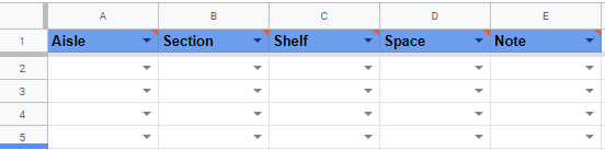
I’m trying to create conditional formatting based on the following spreadsheet:

My intention is that if Space is not empty and Note is, the cell will glow red with anger. I’m using the following formula for the conditional formatting: =and(if(isblank(D2),"FALSE","TRUE"),if(isblank(E2),"TRUE","FALSE"))

Looks great, but that only works for cell E2. How can I drag the conditional formatting down through the rest of the (3000) cells? When I drag the conditioning down now, every cell is conditional on D2 and E2, rather than, for example, cell E3 being conditional on D3 and E3.

Thanks!