I am building a personal finances worksheet. I have a solid pivot table that shows profit/loss for a given date range.
Question 1: How can I show a column (or a separate sheet) that shows monthly averages based on my slider’d date range?
Here’s where I have succeeded:
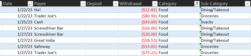
Database Table with accounts, dates, transactions, categories, etc.

Pivot Table with date slider, works as expected to generate PL reports on a date range
In the Pivot Table, I included some calculated boxes:
- Start/End dates pivot table using Min & Max dates in a MMM YYYY format. This is what I used to create the title in yellow.
(Question 2: Can I pull the range title from the slider? E.g. “2022”, “Q1 2022”) - Number of months:
=ROUNDUP(YEARFRAC($E$4,$F$4)*12,0)This is the number to divide by for monthly averages, obvi.
(Question 3: Again, is there a better way to get this from the pivot table itself?)
Here’s what’s not working:

To get the final column, I used a simple calculated field with /12. This works fine for a date range of 12 months, but the other values are useless. I couldn’t figure out a way to pull the number of months (from the Slider) into the calculate field.
How can I use the above breakdown, ideally with columns showing Years Quarters Dates (Months) and each value showing a monthly average?
Alternatively, I would be ok with a final column in my original Pivot Table showing these averages, but I can’t seem to get that number of months variable into a calculated field.

